Univariate analysis
In univariate analysis we explore each variable by itself
Ratio variables
For ratio variables the function plot_univariate_continuous
source
plot_univariate_continuous
 plot_univariate_continuous (df:pandas.core.frame.DataFrame, var:str,
                             var_name:str, ax)
df
DataFrame
Data
var
str
Variable to plot
var_name
str
Variable name
ax
Axes on which to draw the plot
To see the function in action we use the diamonds dataset provided with seaborn
= sns.load_dataset('diamonds' )
0
0.23
Ideal
E
SI2
61.5
55.0
326
3.95
3.98
2.43
1
0.21
Premium
E
SI1
59.8
61.0
326
3.89
3.84
2.31
2
0.23
Good
E
VS1
56.9
65.0
327
4.05
4.07
2.31
3
0.29
Premium
I
VS2
62.4
58.0
334
4.20
4.23
2.63
4
0.31
Good
J
SI2
63.3
58.0
335
4.34
4.35
2.75
This dataset only includes variables with two levels of measurement (ratio and ordinal), the variables can be classified as,
= ['carat' , 'depth' , 'table' , 'price' , 'x' , 'y' , 'z' ]= ['cut' , 'color' , 'clarity' ]
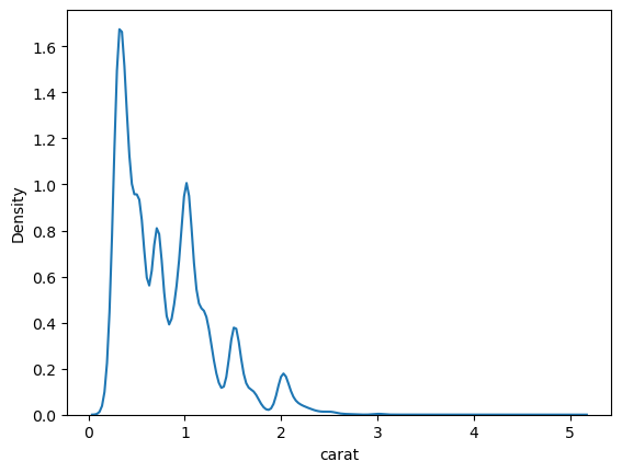
The density plot of the carat feature is
= diamonds, x= 'carat' );
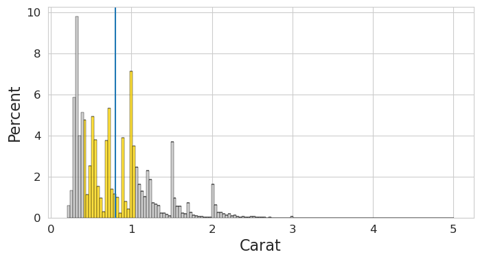
We create an axis in the whitegrid style and call plot_univariate_continuous
with sns.axes_style('whitegrid' ):= plt.subplots(figsize= (8 ,4 ))'carat' , 'Carat' , ax);
findfont: Font family ['Century Gothic'] not found. Falling back to DejaVu Sans.
findfont: Font family ['Century Gothic'] not found. Falling back to DejaVu Sans.
The resulting figure shows an histogram plot made using seaborn.histplot with stat='percent'. It includes a vertical line drawn at the mean of the data and uses colors to distiguish three groups: the first quartile, the fourth quartile and the second and third quartile (together)
Ordinal features
Each of the ordinal features have the following categories ordered from best to worst,
for feat in diamonds_ordinal:print (f'Categories in { feat} :' )print (diamonds[feat].unique())print (' \n ' )
Categories in cut:
['Ideal', 'Premium', 'Good', 'Very Good', 'Fair']
Categories (5, object): ['Ideal', 'Premium', 'Very Good', 'Good', 'Fair']


Categories in color:
['E', 'I', 'J', 'H', 'F', 'G', 'D']
Categories (7, object): ['D', 'E', 'F', 'G', 'H', 'I', 'J']


Categories in clarity:
['SI2', 'SI1', 'VS1', 'VS2', 'VVS2', 'VVS1', 'I1', 'IF']
Categories (8, object): ['IF', 'VVS1', 'VVS2', 'VS1', 'VS2', 'SI1', 'SI2', 'I1']
Bivariate analysis
The goal is a fuction that can calculate a measure of dependence between all the features in a given dataset.
source
strength_of_assoc
 strength_of_assoc (df:pandas.core.frame.DataFrame, ratio_vars:list=None,
                    ordinal_vars:list=None, nominal_vars:list=None,
                    binary_vars:list=None)
df
DataFrame
Data
ratio_vars
list
None
Columns in df with ratio variables
ordinal_vars
list
None
Columns in df with ordinal variables
nominal_vars
list
None
Columns in df with nominal variables
binary_vars
list
None
Columns in df with binary variables
We say a variable has a ratio level of measurement if it is a variable for which ratios are meaningful. Ratio variables have all the properties of interval variables plus a real absolute zero.
For the diamonds dataset we have
= strength_of_assoc(diamonds, diamonds_ratio)
20
y
z
0.952006
Pearson correlation coefficient
strong
2
carat
price
0.921591
Pearson correlation coefficient
strong
3
carat
x
0.975094
Pearson correlation coefficient
strong
4
carat
y
0.951722
Pearson correlation coefficient
strong
5
carat
z
0.953387
Pearson correlation coefficient
strong
strength_of_assocn (n - 1) / 2 pair of variables where n is the number of ratio variables
assert len (diamonds_rcorr.index) == 21
source
soa_graph
soa_graph (cdf:pandas.core.frame.DataFrame, min_strength:str='strong')
cdf
DataFrame
A dataframe as output by ratio_corr
min_strength
str
strong
Threshold for high correlation
= soa_graph(diamonds_rcorr)
= True )
import numpy as npfrom scipy.stats import chi2_contingency= np.array([[205534 , 302607 ], [33395 , 71466 ]])= np.array([[205534 , 302607 ], [40896 , 63965 ]])= chi2_contingency(table)
Chi2ContingencyResult(statistic=75.75518055236239, pvalue=3.2110752959071082e-18, dof=1, expected_freq=array([[204275.33128766, 303865.66871234],
       [ 42154.66871234,  62706.33128766]]))
AttributeError: 'tuple' object has no attribute 'statistic'